2023年3月上旬

2023-03-01 10:01

开始写论文的引言

2023-03-01 11:30

吃饭

2023-03-01 14:42

继续写引言

2023-03-02 10:22

继续写引言

2023-03-06 20:48:06

1. 回忆了一下怎么使用我的程序。

mkdir build && cd build && cmake ..
make -j32

2023-03-06 22:37:24

• 成功测试发送邮件功能

2023-03-07 00:12:17

• 成功测试计时功能

2023-03-07 10:53:07

• 测试插值算子和延拓算子.
  程序为 test/test_ibm_elerian_larangian_interaction.cpp , 测试通过。
  考虑到计算效率, 目前固体只使用一阶有限元方法求解。

2023-03-07 16:00:50

• 显式浸没边界法, 程序为 test_ibm_disk_driven_explicit.cpp

使用 ImersedBoundaryMethod 类
set_dolfin_solver

2023-03-07 18:02:31

test_ibm_disk_driven_explicit.cpp 能够运行了, 但是流体的边界条件还不知道怎么设置。

可能需要在CPU中设置, 然后传输到GPU中。

2023-03-08 10:09:21

对于直杆弯曲问题, 固定边界有两种方式：

1. 通过Dirichlet条件限制
2. 通过惩罚项约束

先实现第一种方法的显式时间离散。

现在, test_ibm_bended_bar_explicit_constraint.cpp 能够运行了。

2023-03-08 10:28:36

现在体积力的计算没问题了。

代码位置: 06b5d561eee0c173c3b65442c6d4ef7cfa3d29c3
边界标记: https://github.com/shaoyaoqian/shaoyaoqian.github.io/releases/download/## 20230221/boundaries## 20230308112542.vtu
体积力: https://github.com/shaoyaoqian/shaoyaoqian.github.io/releases/download/## 20230221/forces## 20230308112803.vtu

体积力的图片：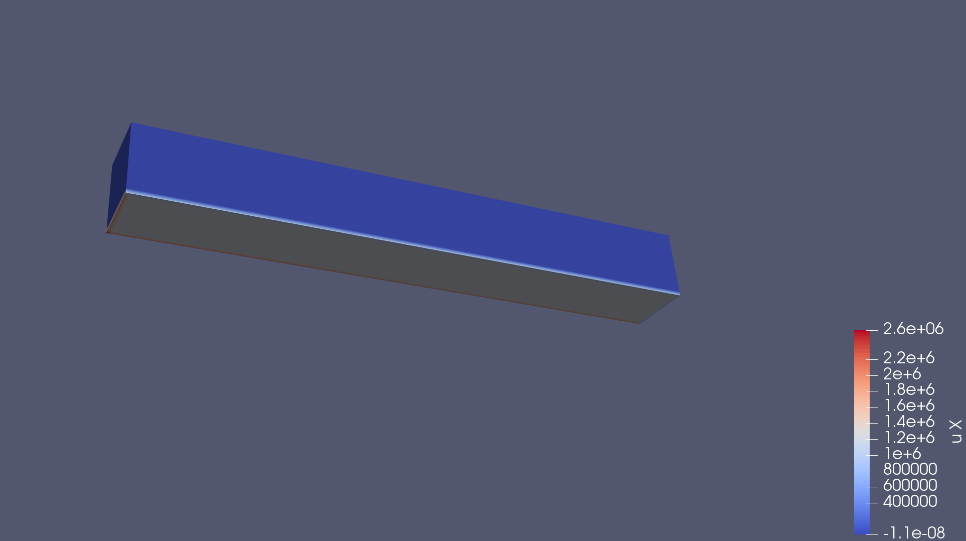

2023-03-08 14:58:31

弯曲直杆问题的显式计算程序 test_ibm_bended_bar_explicit_constraint.cpp 。

1. 测试限制条件。

固体类需要有一个函数, 修改传入的位移或者速度。
GenericSolidSolver 对象几乎是一个无状态的对象, 它不存储当前位置或者初始位置。
真正的数据都存储在 solid_mesh 对象中, 名为_solid_positions , 可以间接通过ImmersedBoundaryMethod获取。

2023-03-08 21:12:57

程序框架的改进

固体求解器不存储以下变量：

1. 固体的当前位置
2. 固体的体积力
   固体求解器根据传入的固体的当前位置计算出固体的体积力。但是会存储一些与模型相关的数据，例如：
3. 边界条件存储在boundaries变量中
4. 当前时刻和时间步长
5. 其他与模型相关的变量，例如本构参数，电势等等。

ImmersedBoundaryMethod 中更新 solid solver 位置的函数也不再有用，因此一并删去。

ImmersedBoundaryMethod 增加了限制固体位移的函数。

2023-03-08 21:30:07

写论文的引言

2023-03-09 10:00:34

完成了引言的参考文献

2023-03-09 11:07:06

测试

带约束条件的直杆弯曲算例
test_ibm_bended_bar_explicit_constraint.cpp 的运行结果

参数：

1. 固体网格的坐标
   (0.45, 0.45, 0.1)
   (0.55, 0.55, 0.9)
2. 网格剖分
   {4, 4, 32};
3. 流体粘性、密度、时间步长：
   double nu = 0.01;
   double rho = 1.0;
   double dt = 0.0001;
4. 背景网格
   int3 dim_bg = {65, 65, 65};
   double3 dh_bg = {0.0, 0.0, 0.0};
   double3 box_size_bg = {1.0, 1.0, 1.0};

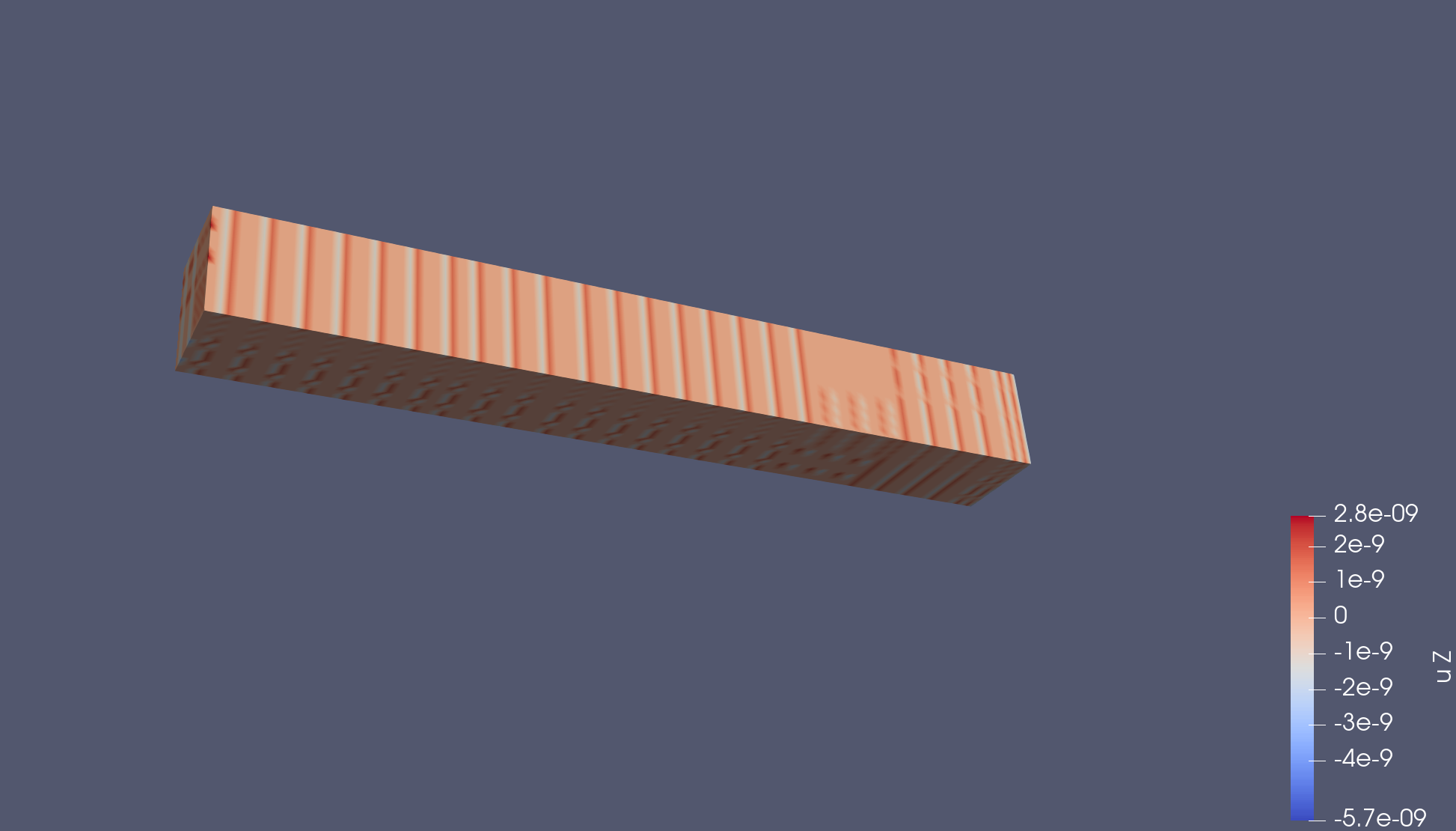
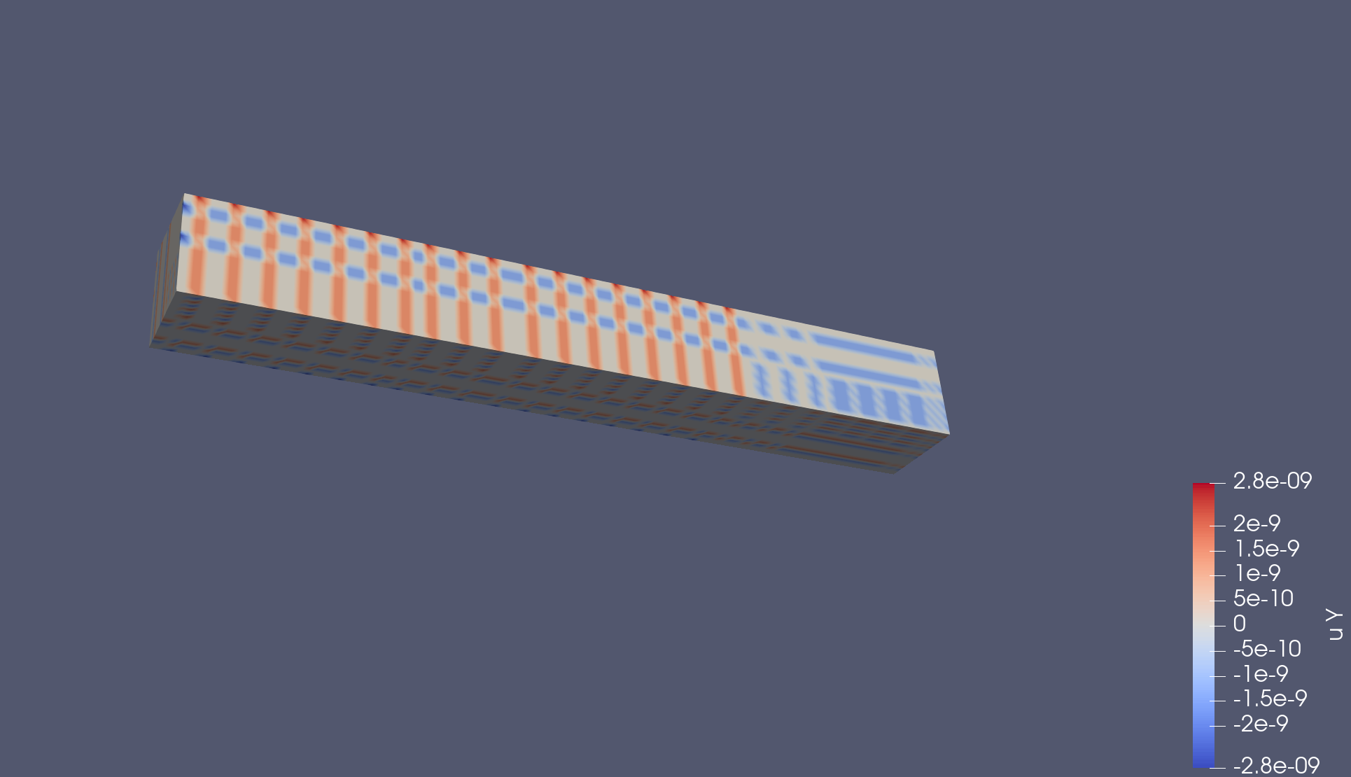
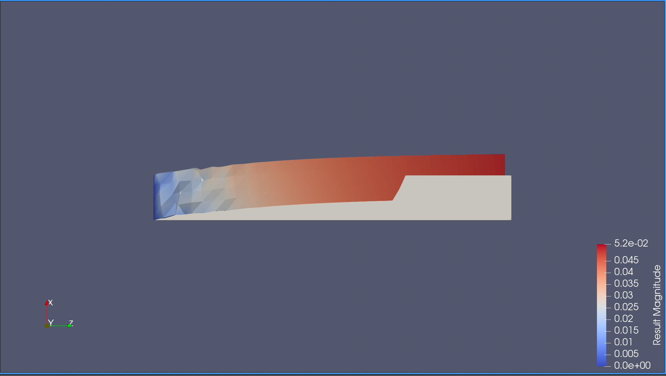
不稳定，可以看到t=0.298时刻的运行结果：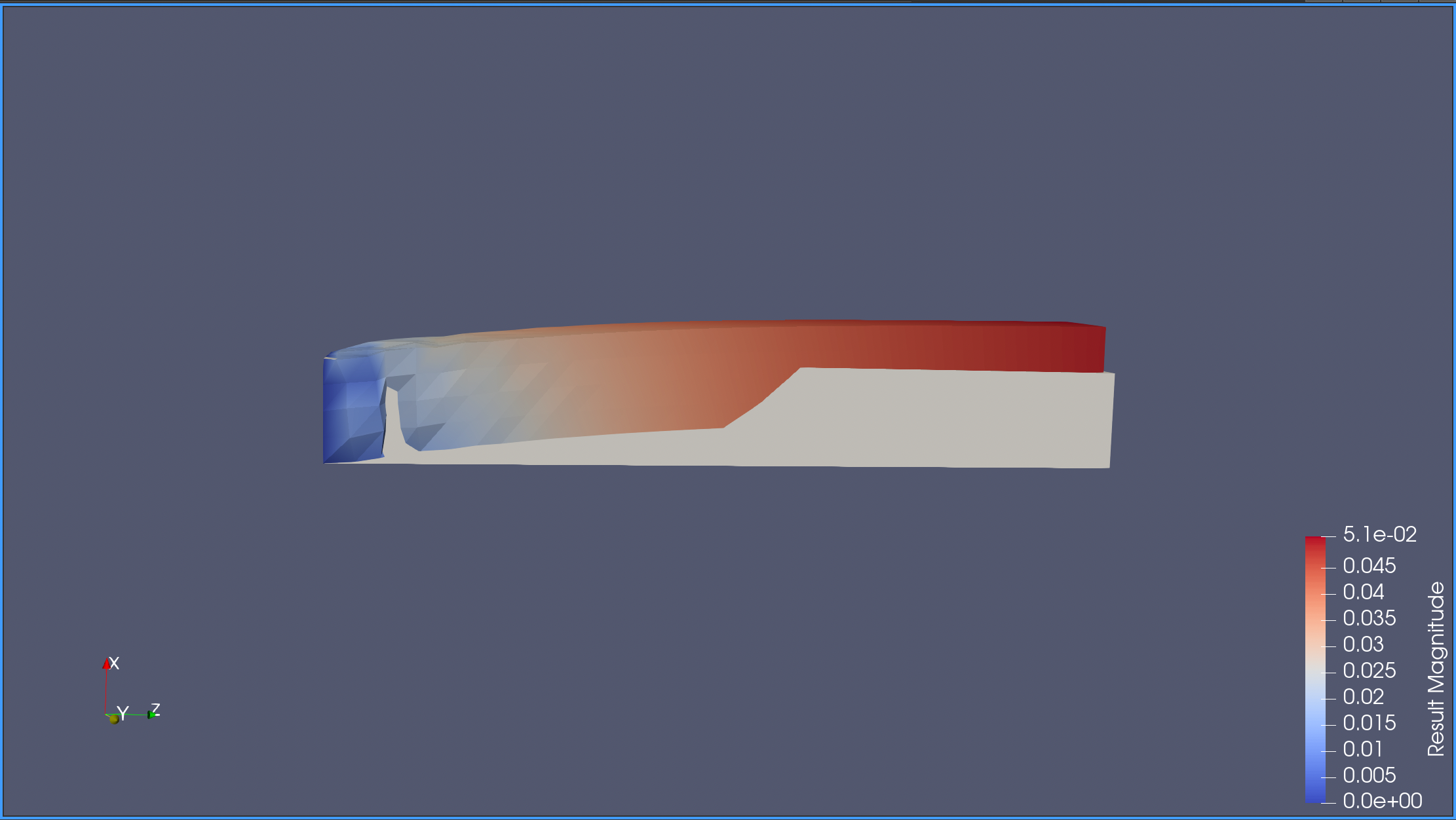

计算结果

https://github.com/shaoyaoqian/shaoyaoqian.github.io/releases/download/20230221/bended_bar_020230309111559.vtu

2023-03-09 11:39:40

应变能函数中加入不可压项

kappa = 100000.0
J = det(F)
kappa * (J**2 - 1 - 2*ln(J))

2023-03-09 17:05:14

加入了不可压项，时间步长仍为$0.0001$，仍旧不稳定，这在预料之中。

代码位置

451c31458906e2d2c158fc404c4824418cb3067e

结果

问题

1. 边界条件可能没有在计算固体的体积力前施加
2. 不可压边界条件不起作用

2023-03-09 20:11:49

问题一：不可压条件

固体的不可压条件可以通过两种方法施加，第一种是拉格朗日乘子法，另一种是通过惩罚项强制$\text{det}(\mathbb{F})=1$满足。一般来说，只要选取其中一种即可。浸没边界法中，不可压条件自然存在。整个计算区域的速度场满足无散度条件，相当于使用了拉格朗日乘子法。但是速度经过插值算子传递到固体区域后，无散度边界条件可能不精确满足，因此需要对固体额外施加不可压条件。以后可以看看文章A monolithic projection framework for constrained FSI problems with the immersed boundary method 是怎么施加约束条件的。

问题二：固体位移的Dirichlet边界条件

有两种方法。第一种是每个时间步后将固体强制拉回原位，第二种是惩罚项。目前发现第一种方法不行。张心欣是用的第一种方法，可能是因为它使用的固体本构简单吧，所以他的没问题。IBAMR一直使用的是第二种方法。

2023-03-10 09:25:49

计划

1. 符号表
2. 完成浸没有限元方法的数学描述

2023-03-10 10:08:57 查看结果

代码位置

168394afa3200c5016eadc8bbfdf21b2b5b2d4cd

参数

int3 dim = {4, 4, 32};
dolfin::Point p2(0.45, 0.45, 0.1);
dolfin::Point p3(0.55, 0.55, 0.9);

double nu = 0.01;
double rho = 1.0;
double dt = 0.00001;
int3 dim_bg = {65, 65, 65};
double3 dh_bg = {0.0, 0.0, 0.0};
double3 box_size_bg = {1.0, 1.0, 1.0};

# Constituitive parameters
C = 20000.0  # dyn/cm^2 (2kPa)
bf = 8.0
bt = 2.0
bfs = 4.0

kappa = 1e4 # Penalty for incompressibility
beta = 1e4  # Penalty for boundary conditions

# Boundary markers
bottom   = 2
fixed    = 1

# Pressure
pressure = 40

结果

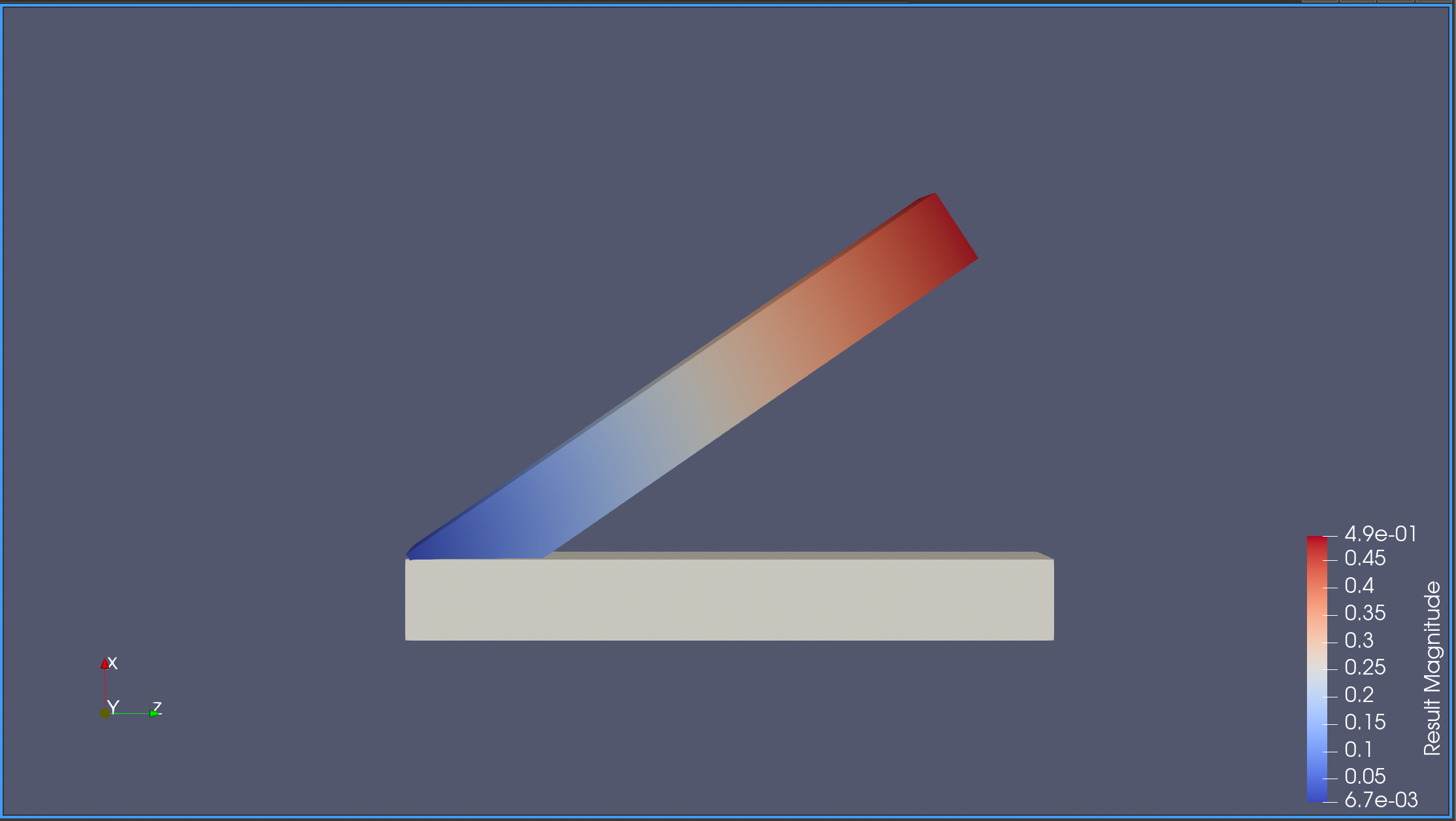
数据

https://github.com/shaoyaoqian/shaoyaoqian.github.io/releases/download/20230221/position00019920230310101333.vtu

问题

1. 惩罚项不够大
2. 直杆没有向正上方偏移

2023-03-10 10:23:34 符号表

以下是本论文中使用的符号的非详尽列表。我们将采用粗体字符表示矢量的惯例。

欧拉描述

	Explanation	中文解释
$\Omega$	An open subset of $\mathbb{R}^n$	背景区域
$\partial \Omega$	boundary of $\Omega$	区域边界
$\mathbf{u}$	Velocity field	速度场
$p$	Pressure field	压强场
$\mathbf{n}$	Unit vector normal to $\partial \Omega$	单位外法向
$\nabla\cdot\mathbf{u}$	Divergence of $\mathbf{u}$	速度散度
$\nabla\mathbf{u}$	Gradient of $\mathbf{u}$	速度梯度
$\Delta\mathbf{u}$	Laplacian of u, defined by $\Delta=\nabla\cdot\nabla$	拉普拉斯算子
$\langle\cdot,\cdot\rangle$	$L^2$-inner product on $\Omega$	$L^2$内积
$|\cdot|_k$	Norm defined by the $H^k$-inner product on $\Omega$ if $k = 0, 1$	$H^{k}$范数
$|\cdot|_2$	Euclidian norm	欧几里得范数
$\mathbf{x}$	$\mathbf{x}=(x_1,x_2,x_3)$ Eulerian coordinates	欧拉坐标

拉格朗日描述

参数

	Explanation	中文解释
$\mu$	(Dynamic) Viscosity	动力粘性
$\rho$	Density	密度
$\nu$	Kinematic viscosity, defined as nu:=mu//rho	运动粘性
$\Delta t$	Timestep	时间步长
$Re$	Reynolds number	雷诺数
$h$	Discretization parameter[1]	空间离散参数

矩阵的性质

	Explanation	中文解释
$L^2(\Omega)$	Space of square-integrable functions on $\Omega$	$\Omega$上的平方可积函数
$H^k(\Omega)$	Space of $L^2$-functions on $\Omega$ with derivatives up to order $k$ which are also in $L^2(\Omega)$	$H^{k}$空间
$H_0^k(\Omega)$	Space of functions in $H^k(\Omega)$ which equal zero on $\partial \Omega$	$H^1$空间
$H^{-1}$	Dual space of $H^1$	$H^1$的对偶空间

固体力学

	Explanation	中文解释
$\boldsymbol \sigma$	The Cauchy stress tensor	柯西应力张量
$\mathbb{P}$	the first Piola–Kirchhoff stress tensor	第一PK应力张量
$W$	Strain energy density function	应变能密度函数
$E$	Elastic potential energy function	弹性势能函数
$?$	Kinetic energy function	动能函数
$B$	A region in three-dimensional Euclidean point space($\mathbb{R}^n$), called configuration of $\mathcal{B}$	固体的构型
$B_r$	A specific configuration of $\mathcal{B}$	参考构型
$B_t$	Current configutation of $\mathcal{B}$	现时构型，当前构型
$\mathcal{B}$	A body, considered as a set of elements, or particles, or material points, whatever	固体

$\mathcal{X}(\mathbf{X},t)$	bijection mapping between $B_r$ and $B_t$
$\mathbf{X}$	$\mathbf{X}=(X_1,X_2,X_3)$Coordinates of material points at reference configuration	固体粒子在参考构型的坐标
t	current time	当前时间
$T$	total time interval	时间间隔

浸没边界法

$\mathcal{S}(\mathbf{X},t)$	prolongation operation, distribution operator	延拓算子
$\mathcal{J}(\mathbf{\mathbf{X}},t)$	restriction operator, interpolation operator	插值算子

2023-03-10 16:40:37 完成文章的第二章

图1描述了一物体$\mathcal{B}$在固定的背景区域$\Omega$中运动的过程。 物体 $\mathcal{B}$ 所有质点空间坐标的集合称为其构型，记为$B$。$t\in[0,T]$ 表示时间，$B_t$ 表示固体 $\mathcal{B}$ 在 $t$ 时刻的构型，称为现时构型。对任意时间$t$，有唯一的构型$B_t$与之对应，这些构型的集合$\{B_t\}$称为物体$\mathcal{B}$在时间$[0,T]$的运动。$\mathcal{B}_r$表示固体在$t=0$时刻的构型，称为参考构型。$\mathbf{X}$表示物体$\mathcal{B}$任一质点在参考构型中的空间坐标，$\mathbf{X}=$ $\left(X_{1}, X_{2}, \ldots\right)\in B_{r} \subset \mathbb{R}^{d}, d=2,3$ ，称之为拉格朗日坐标。$\mathcal{X}(\mathbf{X},t)$是从$B_r$到$B_t$的映射，映射$\mathcal{X}(\mathbf{X},t)$称为固体从$\mathcal{B}_r$到$\mathcal{B}_t$的形变。$\mathcal{X}(\mathbf{X},t)$ 是定义在参考构型 $B_r$ 上的物理量，以$\mathbf{X}$为自变量，我们称之为拉格朗日描述。区域$\Omega$表示流固耦合系统占据的物理区域，$\Omega/B_t$为流体区域，我们讨论定义在$\Omega$上的方程，不对流体区域进行单独描述。$\mathbf{x}$表示$\Omega$中的任意一点，$\mathbf{x}=\left(x_{1}, x_{2} \ldots\right)\in \Omega \subset \mathbb{R}^{d}, d=2,3$，称之为欧拉坐标。$\mathbf{u}(\mathbf{x},t)$、$p(\mathbf{x},t)$分别表示流固耦合系统的速度场和压力场。

Figure 1 describes the motion of an body $\mathcal{B}$ in a fixed background domain $\Omega$. The set of spatial coordinates of all particles of body $\mathcal{B}$ is called its configuration, denoted by $B$. $t\in[0,T]$ represents time, $B_t$ represents the configuration of body $\mathcal{B}$ at time $t$, which is called the current configuration. For any time $t$, there is a unique configuration $B_t$ corresponding to it. The set of these configurations ${B_t}$ is called the motion of body $\mathcal{B}$ during time $[0,T]$. $B_r$ denotes the configuration of the body at $t=0$, called the reference configuration. $\mathbf{X}$ represents the spatial coordinate of a specific particle in the reference configuration of body $\mathcal{B}$, $\mathbf{X}=\left(X_{1}, X_{2}, X_{3}\right)\in B_{r} \subset \mathbb{R}^{e}$, which is called the Lagrangian coordinate. $\mathcal{X}(\mathbf{X},t)$ is the mapping from $B_r$ to $B_t$, which is called the deformation of the body from $B_r$ to $B_t$. $\mathcal{X}(\mathbf{X},t)$ is a physical quantity defined on the reference configuration $B_r$. We call it the Lagrangian description, with $\mathbf{X}$ as its independent variable. The domain $\Omega$ represents the physical domain occupied by the fluid-solid coupling system. $\Omega/B_t$ denotes the fluid domain. We discuss equations defined on $\Omega$ and do not separately describe the fluid domain. $\mathbf{x}$ represents any point in $\Omega$, $\mathbf{x}=\left(x_{1}, x_{2}, x_{3}\right)\in \Omega \subset \mathbb{R}^{3}$, which is called the Eulerian coordinate.

假设固体和流体均不可压且密度相等，流体为牛顿流体，固体为粘超弹性固体，流固耦合系统的柯西应力张量为

Assuming that both the solid and fluid are incompressible and have equal densities, the fluid is assumed to be a Newtonian fluid and the solid is assumed to be a viscous hyperelastic material, then the Cauchy stress tensor of the fluid-structure coupling system is given by

$$\boldsymbol{\sigma}(\mathbf{x}, t)=\boldsymbol{\sigma}^{\mathrm{f}}(\mathbf{x}, t)+ \begin{cases}\boldsymbol{\sigma}^{\mathrm{e}}(\mathbf{x}, t) & \mathbf{x} \in B_t \\ \mathbf{0} & \mathbf{x}\in\Omega/B_t\end{cases}$$

Here are the meanings of the quantities and variables that appear in the above equations in details.

$$\boldsymbol{\sigma}^{\mathrm{f}}(\mathbf{x}, t)=-p(\mathbf{x}, t) \mathbb{I}+\mu\left[\nabla \mathbf{u}(\mathbf{x}, t)+(\nabla \mathbf{u}(\mathbf{x}, t))^{\mathrm{T}}\right]$$

$$\boldsymbol{\sigma}^{\mathrm{e}}(\mathbf{x}, t)=\boldsymbol{\sigma}^{\mathrm{e}}(\boldsymbol{\mathcal{X}}(\mathbf{X}, t), t) = J^{-1}(\mathbf{X}, t)\mathbb{P}^{\mathrm{e}}(\mathbf{X}, t)\mathbb{F}^{\mathrm{T}}(\mathbf{X}, t)$$

$\mathbb{I}$为单位张量，$\mu$为运动粘性，$\mathbb{F}(\mathbf{X},t)$为形变梯度，$J(\mathbf{X}, t)=\operatorname{det}(\mathbb{F}(\mathbf{X}, t))$，$\mathbb{P}(\mathbf{X},t)$为第一Piola-Kirchhoff应力张量，可以通过对应变能函数$W(\mathbb{F})$求导得到

$\boldsymbol{\sigma}^{\mathrm{f}}(\mathbf{x}, t)$ is the fluid-like component of stress tensor which exits everywehre in $\Omega$, $\mathbf{u}(\mathbf{x},t)$ and $p(\mathbf{x},t)$ represent the velocity field and pressure field of the fluid-solid coupling system, respectively. $\mathbb{I}$ is the identity tensor, $\mu$ is the dynamic viscosity. $\boldsymbol{\sigma}^{\mathrm{f}}(\mathbf{x}, t)$ is the elastic component of stress tensor which only exists in solid domain. $\mathbb{F}(\mathbf{X},t)$ is the deformation gradient, $J(\mathbf{X}, t)=\operatorname{det}(\mathbb{F}(\mathbf{X}, t))$, and $\mathbb{P}(\mathbf{X},t)$ is the first Piola-Kirchhoff stress tensor, which can be obtained by taking the derivative of the corresponding strain energy function $W(\mathbb{F})$

$$\mathbb{P}^{\mathrm{e}}=\frac{\partial W^{\mathrm{e}}}{\partial \mathbb{F}}$$

浸没边界法的控制方程可以通过动量守恒定律和质量守恒定律推导。在求解中，$\boldsymbol{\sigma}^f(\mathbf{x}, t)$需采用欧拉描述，$\boldsymbol{\sigma}^{e}(\mathbf{x}, t)$需采用拉格朗日描述，它们之间通过与delta核函数的积分变换建立起联系。本文采用了Boyce等人推导的方程组。

The governing equations of the Immersed Boundary Method can be derived from the principles of conservation of momentum and mass. When we solve the problem practically, the fluid stress tensor $\boldsymbol{\sigma}^f(\mathbf{x}, t)$ is expressed in Eulerian description, while the solid stress tensor $\boldsymbol{\sigma}^{e}(\mathbf{x}, t)$ is expressed in Lagrangian description. The relationship between them is established through integration with the delta kernel function. Equations derived by Boyce et al. is adopted in this paper.

$$\rho(\frac{\partial \bf{u}}{\partial t}+(\bf{u}\cdot \nabla)\bf{u}) +\nabla p -\mu \Delta \bf{u} = \bf{f}$$

$$\nabla\cdot \bf{u} = 0$$

$$\int_{\bf{B}_{r}}\bf{F}\cdot \bf{V}d\bf{X} =-\int_{\bf{B}_{r}}\mathbb{P} :\nabla \bf{V}d\bf{X}$$

$$\bf{f}(x,t) = \int_{\bf{B}_{r}} \bf{F}(\bf{X},t)\delta(x-\chi(\bf{X},t)d\bf{X}$$

$$\frac{\partial{\chi (\bf{X,t})}}{\partial t} =\int_{\Omega}\bf{u}(x,t)\delta (\chi (\bf{X},t)-x)dx$$

2023-03-11 01:26:50 多孔介质固体的流固耦合

灌注压力的求解

• $M_b$:常数
• $p$：是灌注压力，和流体的压力无关
• $f(J)=\frac{2(J(\mathbf{X}, t)-1-\ln (J(\mathbf{X}, t)))}{(J(\mathbf{X}, t)-1)^2}$
• $E(M,J)$:一个标量，与$m^n$和$J^n$

$$\frac{P^{n+\frac{1}{2}}-P^n}{\triangle t / 2}-M_b f\left(J^n\right) \nabla_{\mathbf{X}} \cdot\left(J^n \mathbb{F}^{-1} \mathbf{K} \mathbb{F}^{-T} \nabla P^{n+\frac{1}{2}}\right)=E\left(M^n, J^n\right)$$

在求解此方程之前，我们先考虑带矩阵系数的泊松方程。

带矩阵系数的泊松方程

带矩阵系数的泊松方程为：

$$-\nabla \cdot(\boldsymbol{A}\nabla u) = f$$

其中，$u$是未知函数，$f$是已知函数，$\boldsymbol{A}$是一个矩阵。其变分形式可以表示为：找到一个函数$u \in H^1(\Omega)$，满足下列变分问题：

$$\int_{\Omega} \boldsymbol{A}\nabla u \cdot \nabla v \;dx = \int_{\partial \Omega} A\nabla u\cdot \mathbf{n} v \;ds+\int_{\Omega} fv \;dx \quad\forall \;v \in H^1(\Omega)$$

其中$\Omega$是定义域，$\partial \Omega$是$\Omega$的边界。若$g=A\nabla u\cdot \mathbf{n}$为已知函数，则能求解。

2023-03-11 12:21:22

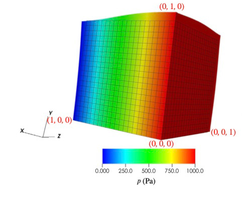
算例1：立方体膨胀 swelling for a cube

背景区域：区域为 $1 \times 1 \times 1 \mathrm{~cm}^3$ ，网格剖分为 $96 \times 96 \times 96$ 。

质疑：背景区域和固体区域一样大么？

固体的位移边界条件：$x=0,y=0,z=0$三个平面的法向位移为零。

源项：$S=0$。

灌注压力：

• $x=0$平面施加与时间相关的压力，$p_{\mathrm{bc}}=10^3\left(1-\exp \left(-t^2 / 0.25\right)\right)$。
• $x=1$平面的压力恒为零。
• 其他平面为零Neumann边界条件。

预期结果：

由于平面$x=0$施加了空隙压力(pore pressure)，立方体会像海绵一样膨胀。

2023-03-11 12:21:44

代码位置

168394afa3200c5016eadc8bbfdf21b2b5b2d4cd

参数

int3 dim = {4, 4, 32};
dolfin::Point p2(0.45, 0.45, 0.1);
dolfin::Point p3(0.55, 0.55, 0.9);

double nu = 0.01;
double rho = 1.0;
double dt = 0.000005;
int3 dim_bg = {65, 65, 65};
double3 dh_bg = {0.0, 0.0, 0.0};
double3 box_size_bg = {1.0, 1.0, 1.0};

# Constituitive parameters
C = 20000.0  # dyn/cm^2 (2kPa)
bf = 8.0
bt = 2.0
bfs = 4.0

kappa = 1e1 # Penalty for incompressibility
beta = 1e7  # Penalty for boundary conditions

# Boundary markers
bottom   = 2
fixed    = 1

# Pressure
pressure = 40

结果

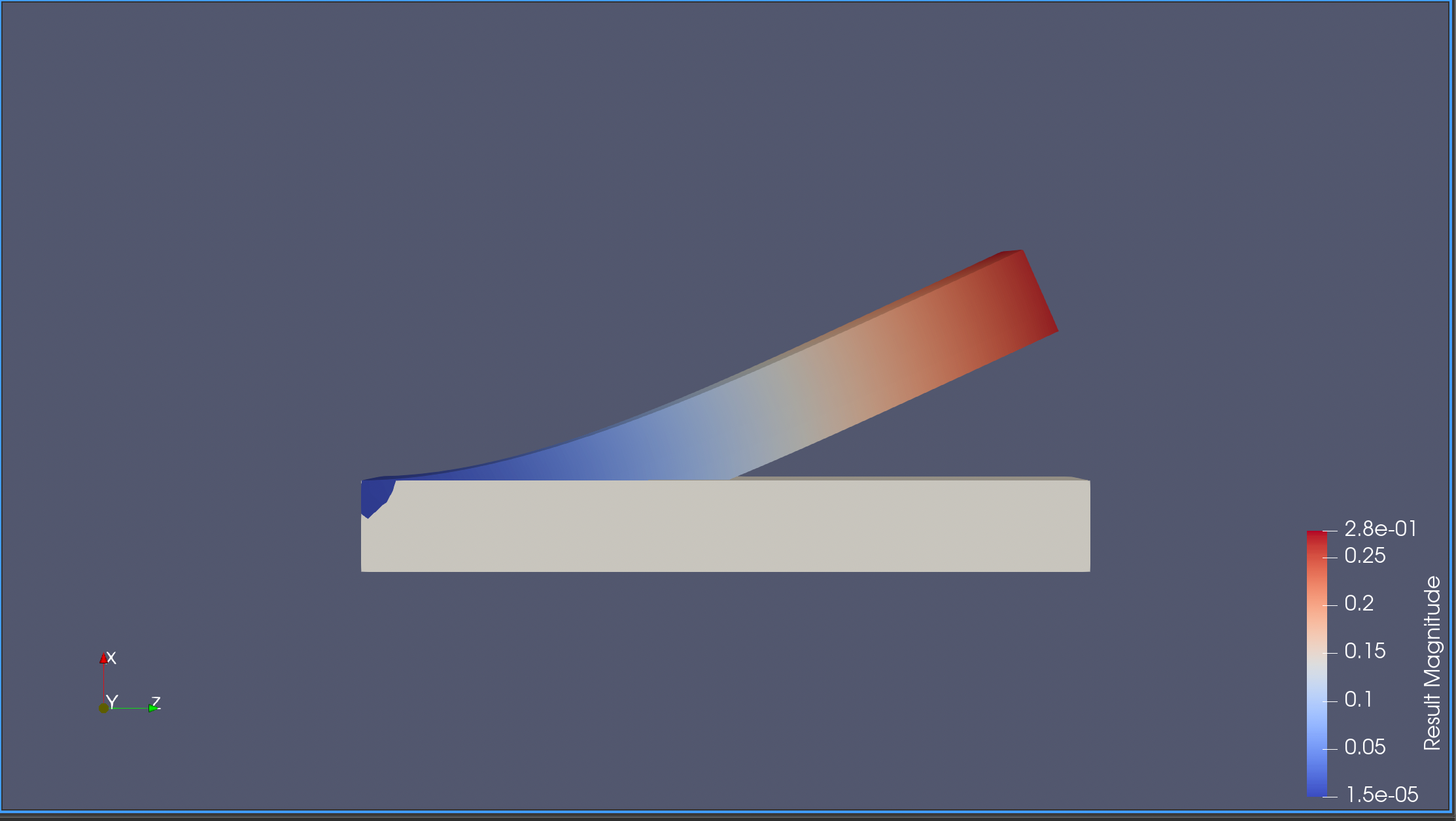
数据

https://github.com/shaoyaoqian/shaoyaoqian.github.io/releases/download/20230221/position00017020230311122948.vtu

问题

1. 直杆没有向正上方偏移
2. 参数kappa过大是否会导致直杆不会弯曲

---

1. Discretization parameter, proportional to the length of the longest edge of an element in a partition of $\Omega$ ↩︎